Solow's model (Solow-Swan model)
1. Basic Structure of the Solow Model
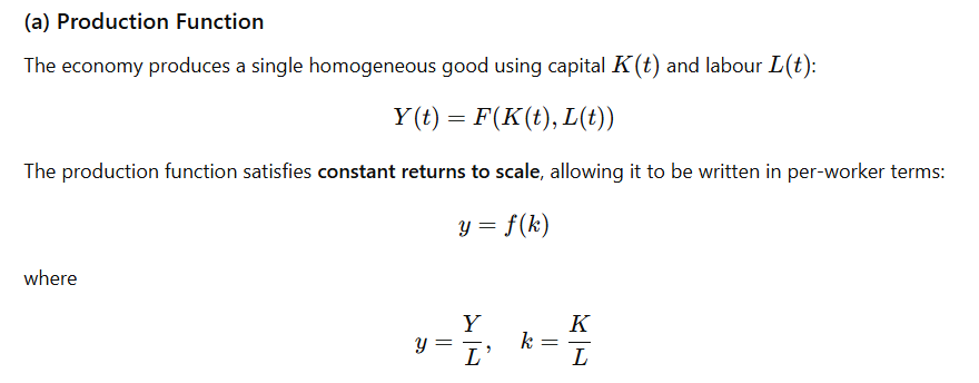 y → output per worker; k = capital per worker.
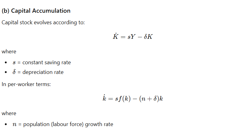
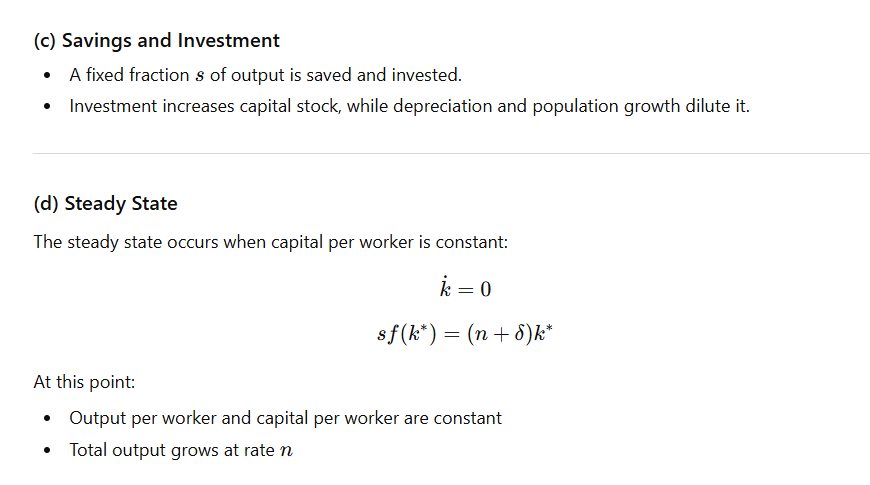
- sf(k) → investment per worker
- Saving creates new capital
- Raises capital per worker
- $delta k$ → depreciation per worker
- Machines wear out
- Reduces capital per worker
- $n k$ → capital dilution
- New workers arrive
- Same capital must be shared among more workers
- Even if total capital stays constant, capital per worker falls
2. Assumptions of the Solow Growth Model
The Solow model rests on several key assumptions, which define its structure and conclusions.
(1) Neoclassical Production Function
Constant returns to scale
Diminishing marginal product of capital
Positive but diminishing marginal productivity of inputs
This ensures convergence to a steady state.
(2) Single Good Economy
- One good is produced and can be used for both consumption and investment.
(3) Constant Saving Rate
Households save a fixed proportion of income.
Saving behaviour is exogenous, not derived from optimisation.
(4) Exogenous Population Growth
Labour force grows at constant rate nnn.
No migration or demographic transitions within the model.
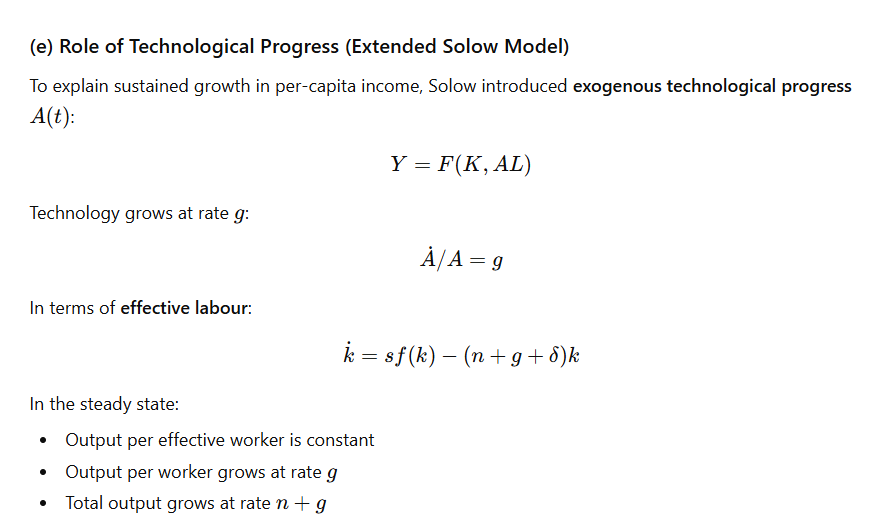
(5) Exogenous Technological Progress
Technology grows at a constant rate ggg.
The model does not explain the source of innovation.
(6) Capital Depreciation
- Capital depreciates at a constant rate δdeltaδ.
(7) Perfect Competition
Factors are paid their marginal products.
No monopoly power or distortions.
(8) Closed Economy
No international trade or capital flows.
Investment equals domestic saving.
(9) No Government Sector
No taxes, public expenditure, or fiscal policy.
Growth is driven purely by private saving and technology.
(10) Full Employment of Resources
All labour and capital are fully employed.
No involuntary unemployment.
3. Implications of the Solow Model’s Structure
Diminishing returns to capital imply that capital accumulation alone cannot sustain long-run growth.
Technological progress is the sole source of long-run per-capita growth.
Poor countries tend to grow faster than rich ones conditional on similar fundamentals (conditional convergence).
Policy variables (saving, population growth) affect levels of income, not long-run growth rates.
4. Significance of the Solow Model
Provides a benchmark framework for growth analysis
Explains cross-country income differences
Introduces the concept of steady-state growth
Forms the basis for modern growth theories, including endogenous growth models
Harrod’s model (Knife-edge model)
Harrod’s Model of Economic Growth
Harrod’s growth model (also called the Harrod-Domar model) is a dynamic Keynesian model that examines the conditions required for an economy to achieve steady growth. It emphasises the knife-edge instability of the growth process.
Harrod distinguishes among three types of growth rates:
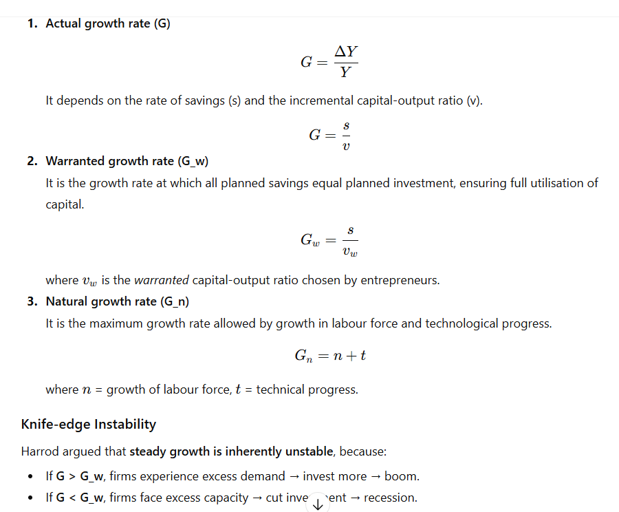
Harrod’s Explanation of Trade Cycles
Harrod’s model implies that business cycles are inherent in the growth process of a capitalist economy. The interaction of the three growth rates generates fluctuations.
(a) Boom Phase
A boom begins when actual growth temporarily exceeds the warranted rate:
High profits raise expectations.
Induced investment increases.
Output and employment rise rapidly.
But the boom cannot continue indefinitely because the natural growth rate (Gn) imposes an upper limit.
(b) Downturn / Recession
Once actual growth falls below the warranted rate:
Firms face unutilized capacity.
They cut investment sharply.
Lower investment leads to reduced output and income.
Because investment is the driving force of growth, even a small drop creates a multiplier-accelerator contraction, producing a recession.
(c) Recovery
The slump persists until:
Undesirable inventory accumulation is corrected.
Capital stock shrinks relative to output needs.
New profitable opportunities emerge.
Then induced investment picks up again, starting a recovery.
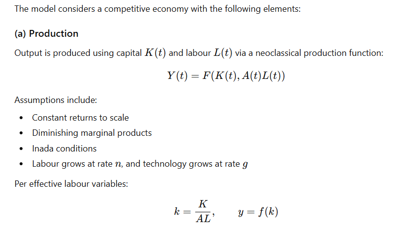
Ramsey–Cass–Koopmans Model (RCK model)
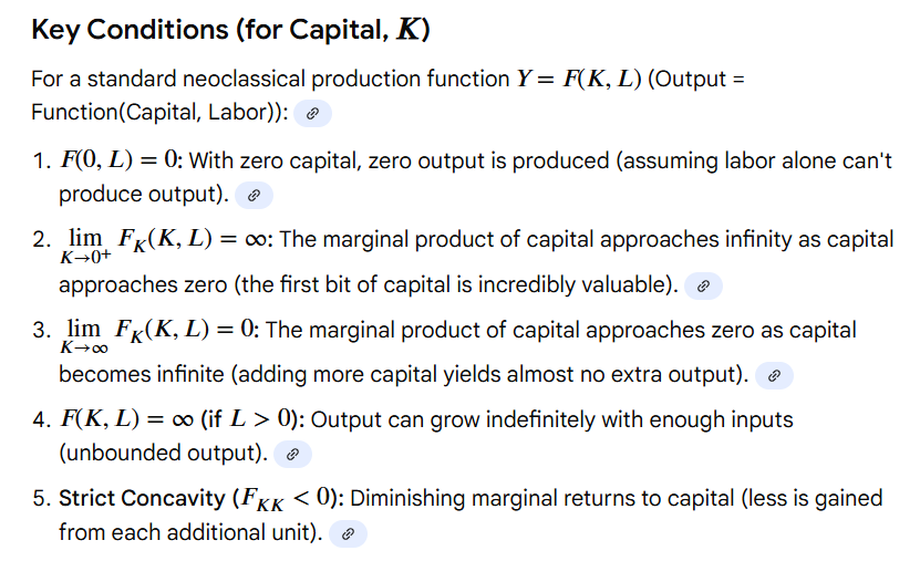
Inada conditions
Inada conditions are mathematical assumptions for production functions (like $Y=F(K,L)$) in economics, named after Ken-ichi Inada, ensuring smooth behavior and stable growth equilibria.
1. Basic Structure and Assumptions
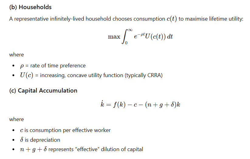
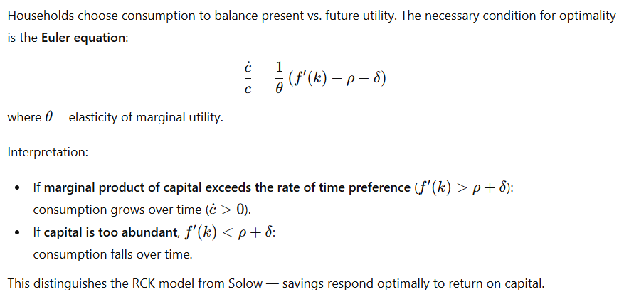
2. Optimal Consumption and the Euler Equation
(a) $ ho$ — Impatience / time preference
Measures how much we prefer today over tomorrow
Higher ρ hoρ = more impatient society
“I want enjoyment now, not later”
(b) $ heta$ — Aversion to inequality across time
Measures how uncomfortable we are with uneven consumption
Higher θ hetaθ = stronger desire to smooth consumption
“I hate big jumps in my standard of living”
(c) r — return on saving
If you save 1 unit today, it grows at rate rrr
More rrr → saving is more attractive
The Euler equation (now in symbols)
$$ rac{dot c}{c} = rac{1}{ heta}(r - ho)$$
This looks scary, but read it in words:
Consumption grows faster when the return on saving exceeds impatience.
Case 1: r>ρ
Saving pays well
Future consumption becomes attractive
Society postpones consumption
Consumption grows over time
Case 2: r<ρ
Society is very impatient
Future isn’t attractive enough
Consume more today
Consumption falls over time
Case 3: r=ρ
Perfect balance
Consumption stays constant
Role of $ heta$ (very intuitive)
θ hetaθ controls how fast consumption responds:
Large θ hetaθ → people strongly prefer smooth consumption
→ consumption changes slowlySmall θ hetaθ → people tolerate inequality
→ consumption changes rapidly
So θ hetaθ is like a shock absorber.
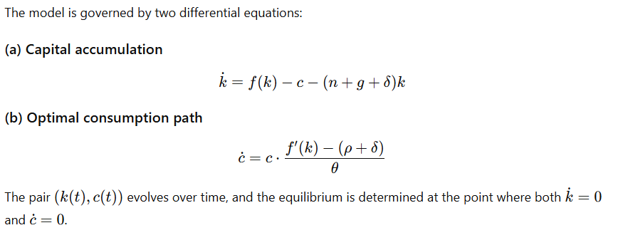
3. Dynamic System of the RCK Model
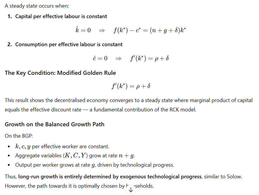
4. Steady-State and Balanced Growth Path (BGP)
5. Transitional Dynamics
A key strength of RCK is its saddle-path stability, meaning:
Only a unique path of (k,c)(k,c)(k,c) leads to the steady state.
Any deviation requires optimal changes in consumption to converge.
Graphically, the saddle path slopes upward, representing the optimal consumption choice given any level of capital.
This allows the model to explain how economies adjust when:
hit by shocks,
starting from different initial capital levels, or
experiencing changes in preferences or technology.
6. Comparison with the Solow Model
| Feature | Solow Model | Ramsey–Cass–Koopmans Model |
|---|---|---|
| Saving Rate | Exogenous | Endogenous (from optimisation) |
| Consumers | Passive | Utility-maximising |
| Dynamics | One equation (capital) | Two equations (capital + consumption) |
| Steady state | Determined by s | Determined by preferences + technology |
| Welfare analysis | Impossible | Possible |
The RCK model provides microfoundations for the saving rate and thus improves upon Solow.
7. Policy Implications
Interest Rate and Consumption
Higher returns on capital raise consumption growth.Taxation of Capital
Distorts optimality condition f′(k)=ρ+δ, potentially lowering welfare.Savings behaviour
Dependent on time preference: impatient societies save less.Transition policies
Governments can help economies move to the saddle path after shocks.
8. Significance of the RCK Model
Microfoundations for long-run growth
Endogenises savings and consumption decisions
Introduces intertemporal optimisation into macroeconomics
Explains transitional dynamics better than Solow
Forms basis for modern macro models (e.g., DSGE, endogenous growth theory)
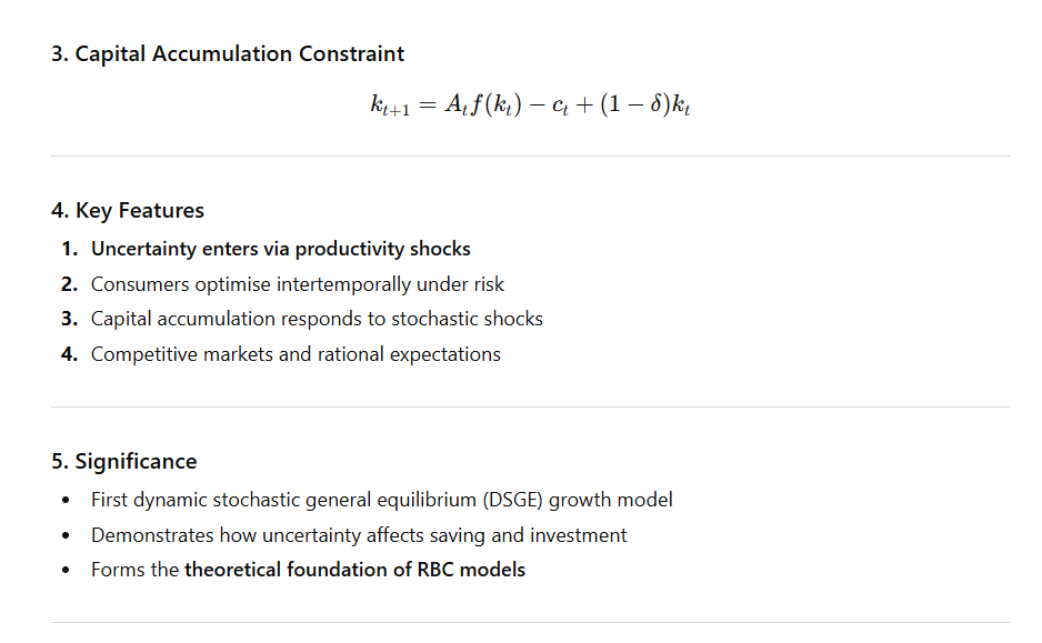
Brock-Mirman growth model
The Brock–Mirman model (1972) is one of the earliest stochastic optimal growth models and is considered a precursor to the Real Business Cycle (RBC) framework. It extends the Ramsey–Cass–Koopmans model by introducing uncertainty through stochastic productivity shocks.
Basic structure

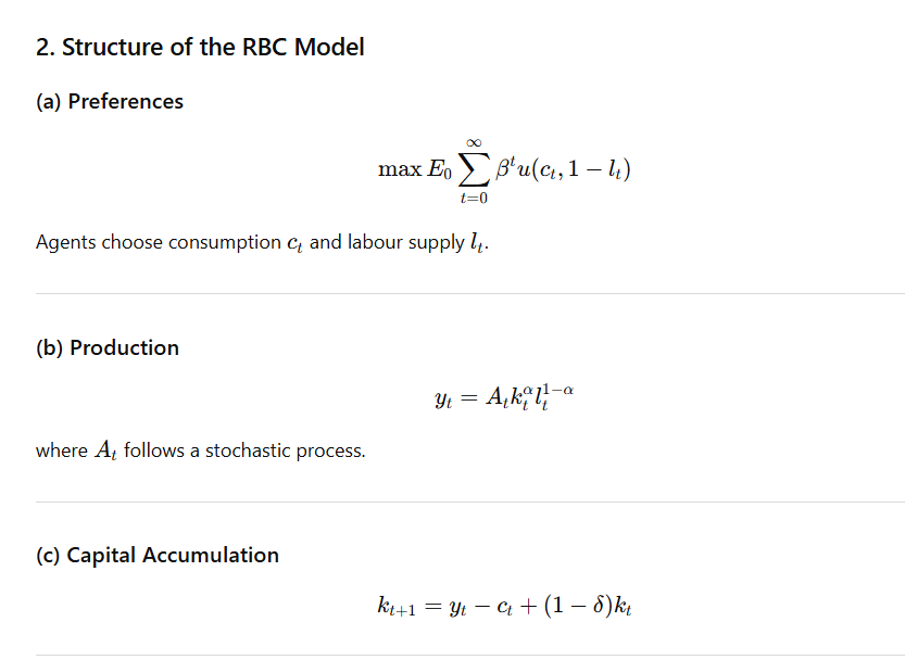
Real Business Cycle (RBC) Model
The Real Business Cycle model, developed by Kydland and Prescott (1982), explains economic fluctuations as optimal responses to real (technology) shocks in a perfectly competitive economy. Business cycles are viewed as efficient outcomes, not failures.
1. Core Assumptions of the RBC Model
Representative agent maximising lifetime utility
Perfect competition in goods and factor markets
Flexible prices and wages
Rational expectations
Technology shocks as the primary source of fluctuations
No role for monetary factors in explaining cycles
Structure
3. Mechanism of Business Cycles
Positive Technology Shock
Raises productivity
Increases output and wages
Households supply more labour
Investment rises
Economic expansion occurs
Negative Technology Shock
Lowers productivity
Reduces labour demand and output
Investment falls
Economy enters recession
Thus, business cycles arise from optimal responses to real shocks, not from market imperfections.
4. Key Results of RBC Models
Fluctuations are Pareto-efficient
No need for stabilization policy
Business cycles are equilibrium phenomena
Labour supply variation explains output volatility
Persistence arises through capital accumulation
5. Policy Implications
Countercyclical policies are unnecessary or harmful
Monetary policy has little real effect
Focus should be on productivity-enhancing reforms
6. Criticisms of RBC Models
Overemphasis on technology shocks
Cannot explain involuntary unemployment
Assumes unrealistic labour supply elasticity
Ignores nominal rigidities
Weak empirical evidence for large technology shocks
Kaldor’s model vs. Pasinetti’s model
Nicholas Kaldor and Luigi Pasinetti belong to the Cambridge (Keynesian–Neo-Ricardian) tradition of growth theory. While Pasinetti builds upon Kaldor’s framework, the two models differ significantly in their assumptions and conclusions regarding saving behaviour, income distribution, and growth.
| Basis of Comparison | Kaldor’s Model | Pasinetti’s Model |
|---|---|---|
| Basic Approach | Keynesian growth model linking growth with income distribution | Extension and correction of Kaldor’s model |
| Classes in Economy | Two classes: workers and capitalists | Same two classes |
| Saving Behaviour | Workers do not save; only capitalists save | Both workers and capitalists save |
| Saving Rates | Single saving rate out of profits | Different saving rates for workers and capitalists |
| Determinant of Growth | Growth determined by capitalists’ saving and investment | Growth independent of workers’ saving |
| Role of Income Distribution | Profit share adjusts to ensure equality of saving and investment | Profit share depends only on capitalists’ saving |
| Ownership of Capital | Capital owned only by capitalists | Workers can also own capital |
| Key Result | Higher profit share raises saving and growth | Workers’ saving does not affect long-run growth |
| Stability Condition | Requires profit share adjustment | More robust and theoretically consistent |
| Major Contribution | Links growth with functional income distribution | Resolves logical inconsistency in Kaldor’s model |
Explanation in Words (for Examiners)
Kaldor’s model assumes that workers consume all wages while capitalists save all profits. Growth depends on the profit share, which adjusts to generate the required saving for investment.
Pasinetti criticizes this assumption, arguing that workers also save and accumulate capital. Surprisingly, he proves that even when workers save, the long-run rate of growth and profit share are determined solely by capitalists’ saving behaviour.
This result is known as the Pasinetti Theorem, and it strengthens the logical foundations of the Cambridge growth models.
Endogenous growth theory
Endogenous Growth Theory explains long-run economic growth as the result of internal forces within the economy, rather than exogenous technological progress as assumed in the Solow model. It emerged in the 1980s, mainly through the works of Paul Romer and Robert Lucas, to explain sustained growth without diminishing returns.
A. Brief Account of Endogenous Growth Theory
2. Core Idea
The central proposition is that knowledge, human capital, innovation, and learning are produced within the economy through purposeful investment decisions. These factors generate increasing returns and positive externalities, enabling sustained per capita growth.
3. Role of Knowledge and Technology
Knowledge is treated as a non-rival and partially non-excludable good, meaning its use by one firm does not reduce availability to others. This leads to spillover effects that raise productivity across the economy.
4. AK Model
A simple representation is the AK model:
$$Y=AK $$ Here, A captures technology and institutional efficiency, while K includes both physical and human capital. Since marginal returns to capital do not diminish, continuous capital accumulation leads to sustained growth.
5. Romer’s Model (1986, 1990)
Romer emphasized research and development (R&D) and innovation. Firms invest in knowledge creation, which increases the stock of ideas. Knowledge spillovers ensure increasing returns at the aggregate level, sustaining growth.
6. Lucas Model (1988)
Lucas highlighted human capital accumulation through education and learning-by-doing. Individual investment in skills raises not only private productivity but also social productivity through externalities.
7. Role of Externalities
Endogenous growth relies heavily on positive externalities from education, innovation, and learning. These externalities offset diminishing returns to capital at the economy-wide level.
8. Policy Sensitivity
Unlike exogenous models, long-run growth in endogenous theory is policy-dependent. Government policies affecting education, R&D, trade, and institutions can permanently influence growth rates.
B. Importance of Endogenous Growth Theory in the Present Scenario
9. Explaining Persistent Growth Differences
The theory explains why some countries grow faster than others due to differences in human capital, innovation capacity, and institutions, rather than only capital accumulation.
10. Relevance for Knowledge-Based Economies
In today’s economy, growth is driven by technology, digitalisation, AI, and innovation, aligning closely with endogenous growth mechanisms.
11. Role of Education and Skill Development
With rapid technological change, continuous skill upgradation and education are crucial for productivity and growth, as highlighted by Lucas’ human capital model.
12. Innovation and R&D-Led Growth
Global competition makes innovation and R&D investment essential. Endogenous theory justifies public support for research due to knowledge spillovers.
13. Policy Guidance for Developing Economies
For developing countries, the theory supports investment in education, health, infrastructure, and institutions rather than relying solely on capital accumulation.
14. Globalisation and Trade
Trade openness enhances technology diffusion and learning, reinforcing endogenous growth through larger markets and innovation incentives.
15. Addressing Middle-Income Trap
Endogenous growth provides insights into escaping the middle-income trap by shifting from factor-driven to innovation-driven growth.
16. Inclusive and Sustainable Growth
Human capital–led growth promotes inclusion by expanding employment opportunities and improving productivity across sectors.
17. Long-Term Growth and Sustainability
Since physical capital faces limits, sustained long-term growth in the modern era depends on continuous productivity improvements, as emphasised by endogenous growth theory.
Schumpeter’s theory of capitalist development through innovations.
1. Role of Innovation
For Schumpeter, innovation is the fundamental force driving economic development. It involves introducing:
New products
New methods of production
New sources of raw materials
New markets
New forms of organisation
These innovations break the existing circular flow and create new opportunities for profit.
2. The Entrepreneur as the Agent of Change
The key figure in Schumpeter’s model is the entrepreneur, who:
Introduces innovations
Takes risks
Secures credit to finance new production
Disrupts existing patterns of economic activity
The entrepreneur is not a routine manager but a creative destroyer who changes the economic system.
3. Role of Credit and Banks
Innovation requires financing. Schumpeter assigns a central role to the banking system:
Banks create purchasing power by issuing credit
This enables entrepreneurs to acquire resources and implement innovations
Credit expansion thus becomes the engine of capitalist development
Without credit, innovations would not materialize.
4. Creative Destruction
Schumpeter famously stated that capitalism progresses through “gales of creative destruction.”
This means:
New technologies and firms destroy old ones
Existing monopolies are displaced by innovative rivals
Economic structures evolve continuously
Creative destruction explains why capitalism is dynamic but also unstable.
5. Business Cycles and Innovation Waves
Schumpeter linked innovations to business cycles:
Innovations occur in clusters, not individually
A major innovation (e.g., railway, electricity, IT) triggers investment, expansion, and a boom
As the innovation diffuses, profit opportunities decline → slowdown
Eventually leads to recession until new innovations emerge
Thus, capitalist cycles are endogenous, not the result of external shocks.
6. Long-Run Capitalist Development
Schumpeter argued that long-run development is a cumulative process:
Innovations raise productivity
Productivity growth increases income and employment
New industries emerge while older ones decline
Capitalism evolves through successive technological revolutions
This makes development non-linear and transformational.
7. Criticisms
Overemphasis on entrepreneurial role – ignores institutional and social factors.
Cyclical theory too dependent on innovation clusters – empirical debate.
Does not explain why innovations originate at specific times or places.
Assumes easy credit creation and downplays financial constraints.
Despite these critiques, Schumpeter’s insights remain highly influential.
Harrod’s classification of technical change. How does it differ from Hicks’ classification
Technical change refers to improvements in production methods that raise output from given inputs. Harrod and Hicks provide two influential ways of classifying technical progress, based on how technology affects factor productivity, factor proportions, and output–capital ratio.
1. Harrod’s Classification of Technical Change
Harrod (1948) classified technical progress on the basis of its effect on the capital–output ratio (v) when the economy grows at a steady rate. His classification is linked to growth neutrality — whether technical change maintains warranted growth conditions.
Harrod identifies three types of technical change:
(a) Harrod-Neutral (Labour-augmenting) Technical Change
Also called labour-saving or Harrod-neutral progress.
It increases labour efficiency, leaving capital productivity unchanged.
Effective labour becomes L(1+λ)L(1 + lambda)L(1+λ).
The capital–output ratio remains constant, preserving steady growth.
This is the form of technical change compatible with Harrod’s “warranted growth.”
(b) Capital-saving Technical Change
Increases the productivity of capital relative to labour.
For a given output, less capital is needed.
The capital–output ratio falls.
Raises profitability and can accelerate growth.
(c) Capital-using (or Capital-intensive) Technical Change
Requires more capital per unit of output.
The capital–output ratio rises.
Can slow growth unless accompanied by higher saving or investment.
Key Point:
Harrod’s classification is based on how technical change affects the capital–output ratio, which is central to his growth dynamics.
2. Hicks’ Classification of Technical Change
Hicks (1932) classified technical progress based on its effect on factor proportions, especially the marginal products of labour and capital along an isoquant.
Hicks identifies three types:
(a) Hicks-neutral Technical Change
Increases the marginal products of both capital and labour in the same proportion.
Leaves the ratio of marginal products unchanged.
Isoquants shift inward symmetrically.
(b) Labour-saving Technical Change
Raises the marginal product of capital relative to labour.
Firms substitute capital for labour.
Isoquants tilt, indicating more capital-intensive techniques.
(c) Capital-saving Technical Change
Raises the marginal product of labour relative to capital.
Firms substitute labour for capital.
Key Point:
Hicks classifies technical change by its substitution effects between labour and capital on an isoquant.
3. Differences Between Harrod and Hicks
| Basis | Harrod’s Classification | Hicks’ Classification |
|---|---|---|
| Underlying Concept | Capital–output ratio (v) and growth neutrality | Isoquant analysis and factor substitution |
| Focus | Effect of technology on steady growth | Effect of technology on marginal products and factor proportions |
| Definition of Neutrality | Neutral if v remains constant (labour-augmenting) | Neutral if MPK/MPL ratio unchanged |
| Relevance | Long-run macro growth theory | Production theory and microeconomics |
| Types Identified | Harrod-neutral (labour-augmenting), capital-saving, capital-using | Hicks-neutral, labour-saving, capital-saving |
| Implication of Neutrality | Only labour-augmenting technical change maintains steady growth | Neutral progress does not bias factor usage |
| Economic Meaning | Compatibility with warranted growth path | Changes in technology that alter input substitutability |
Government Failure
Government failure refers to situations where government intervention intended to correct market failure leads instead to inefficient allocation of resources, welfare loss, or unintended harmful outcomes.
1. Concept of Government Failure
Government failure occurs when:
Public policies do not achieve their intended goals,
Policies lead to misallocation of resources,
Social welfare is reduced rather than improved,
Costs of intervention exceed the benefits.
It stems from limitations in information, incentives, administration, and political processes.
2. Causes of Government Failure
(a) Imperfect Information
Governments often lack the detailed information needed to design efficient policies.
Example: Incorrect minimum support prices → distorted production patterns.
(b) Bureaucratic Inefficiency
Bureaucracies may be slow, wasteful, or driven by procedural rules instead of efficiency.
(c) Political Incentives
Policies may cater to vote banks, interest groups, or political bargaining, not social welfare.
Example: Subsidies continued despite inefficiency.
(d) Regulatory Capture
Industries influence regulators to frame rules that favour them rather than consumers.
(e) Moral Hazard and Corruption
Government programmes may encourage rent-seeking or leakages (e.g., corruption in welfare schemes).
(f) High Administrative Costs
Monitoring, enforcement, and compliance costs may exceed the welfare gain.
(g) Time Lags
Delay between policy design and implementation reduces effectiveness (e.g., fiscal policy lags).
3. Examples of Government Failure
Inefficient public enterprises with persistent losses
Fertilizer, electricity, and fuel subsidies leading to fiscal stress
Price controls causing shortages or black markets
Poorly targeted welfare schemes
Excessive regulation reducing innovation (“license raj”)
These illustrate that even well-intended interventions may create distortions.
5. Key Differences Between Market Failure and Government Failure
| Aspect | Market Failure | Government Failure |
|---|---|---|
| Definition | Inefficiency arising from market forces | Inefficiency arising from government intervention |
| Cause | Externalities, public goods, monopoly, imperfect information | Bureaucratic inefficiency, political incentives, poor design, corruption |
| Source of Failure | Private decision-making | Public decision-making |
| Corrective Mechanism | Government intervention | Policy reform, decentralization, market-based tools |
| Outcome | Welfare loss, inefficient allocation | Waste, distortions, fiscal burden, unintended consequences |
Behavioural Development Economics
Behavioural Development Economics has emerged as an important field that integrates insights from psychology, behavioural economics, and experimental evidence into the study of development. It challenges the assumptions and policy prescriptions of Traditional Development Economics by highlighting how real human behaviour diverges from rational, utility-maximising models.
1. Traditional Development Economics: Key Features
Traditional Development Economics (1950s–1990s), influenced by neoclassical and structuralist approaches, is based on the following assumptions:
(a) Rationality
Individuals are assumed to be fully rational, forward-looking, and consistent in decision-making.
(b) Perfect Information or Well-understood Constraints
Agents are assumed to know prices, risks, and consequences.
(c) Stable Preferences
Preferences do not change with context or framing.
(d) Focus on Structural Constraints
Development outcomes are explained by:
market failures
institutional weaknesses
poverty traps
capital shortages
poor infrastructure
Policies emphasised investment, structural reforms, human capital, and market efficiency.
2. Behavioural Development Economics: Key Features
Behavioural Development Economics modifies traditional assumptions by recognising that real-world individuals—especially the poor—face psychological, cognitive, and social constraints.
(a) Bounded Rationality
People have limited capacity to process information. Decisions often rely on rules of thumb.
(b) Present Bias
Individuals disproportionately value immediate rewards over future ones, leading to:
under-saving
under-investment in health and education
procrastination
failure to adopt beneficial technologies
(c) Limited Self-Control
Difficulty in following long-term plans, even when intentions are strong.
(d) Imperfect Information and Misperceptions
People make mistakes, misjudge probabilities, or rely on misleading beliefs.
(e) Social Norms and Peer Effects
Behaviour is shaped by:
social networks
cultural norms
community expectations
(f) Emotional and Psychological Factors
Stress, scarcity, and cognitive load affect economic choices.
(g) Evidence from Field Experiments
Behavioural development economists rely heavily on:
randomised controlled trials (RCTs)
impact evaluations
micro-level data
3. How Behavioural Development Economics Differs from Traditional Development Economics
| Aspect | Traditional Development Economics | Behavioural Development Economics |
|---|---|---|
| Human Behaviour | Fully rational, optimising | Bounded rationality, biases, heuristics |
| Decision-making | Based on prices, incentives, constraints | Influenced by psychology, framing, defaults, norms |
| Sources of Underdevelopment | Market failures, capital shortages, institutions | Cognitive biases, scarcity mindset, lack of self-control |
| Policy Tools | Regulation, investment, subsidies, macro reforms | Nudges, reminders, commitment devices, behavioural incentives |
| Approach to Poverty | Poverty as a resource/income problem | Poverty as a cognitive and behavioural trap |
| Methodology | Theoretical models + macro data | RCTs, behavioural experiments, micro evidence |
| Focus | Structural change, capital accumulation | Individual behaviour, micro-level decision-making |
| Intervention Design | Assumes agents respond predictably to incentives | Designs account for psychological reactions and biases |
4. Examples of Behavioural vs. Traditional Approaches
Savings
Traditional: Increase interest rates, improve banking access.
Behavioural: Automatic savings enrolment, reminders, commitment devices.
Health
Traditional: Build hospitals, reduce prices.
Behavioural: Use default vaccination appointments, small incentives, SMS reminders.
Education
Traditional: Increase school funding.
Behavioural: Provide information nudges, role models, motivational interventions.
Technology Adoption
Traditional: Subsidise new technologies.
Behavioural: Reduce complexity, demonstrate benefits through peer learning.
These examples show how small behavioural nudges can produce large improvements at low cost.
Concept of rights in a multi dimensional perspective
Rights are fundamental claims or entitlements that individuals possess by virtue of being members of society. Rights are multidimensional—that is, they encompass legal, political, social, economic, ethical, and developmental dimensions.
1. Legal Dimension
The legal dimension refers to rights guaranteed by the constitution, laws, and judicial systems. These include:
Fundamental rights (e.g., equality, freedom of speech)
Legal protections against discrimination or injustice
Enforcement mechanisms through courts
This dimension ensures that rights are codified, enforceable, and protected.
2. Political Dimension
Rights also involve active participation in civic and political processes. These include:
Right to vote
Right to contest elections
Freedom of association
Right to protest and express political opinions
Political rights empower individuals to influence governance and hold institutions accountable.
3. Economic Dimension
Economic rights concern access to resources and opportunities necessary for a dignified life:
Right to work
Right to minimum wages
Right to livelihood
Right to fair economic participation
These rights recognise that economic deprivation restricts individual freedoms, and development requires ensuring equitable economic opportunities.
4. Social Dimension
Social rights relate to living conditions and inclusion within society:
Right to education
Right to health
Right to social security
Right to non-discrimination (gender, caste, religion)
They highlight that human well-being is shaped by social structures, institutions, and collective norms.
5. Ethical and Moral Dimension
Rights are grounded in philosophical ideas of:
Human dignity
Justice
Equality
Respect for individual autonomy
This dimension asserts that rights are not merely legal claims but ethical imperatives reflecting universal moral values.
6. Cultural Dimension
Rights also involve recognition of cultural identity and diversity:
Right to language
Right to practise culture, tradition, and religion
Protection of indigenous and minority rights
This dimension emphasises that development must respect cultural plurality.
7. Developmental Dimension
Modern development thinking (UNDP, Amartya Sen) sees rights as central to expanding capabilities and freedoms. This includes:
Freedom from poverty
Freedom from exploitation
Access to opportunities that enhance human capabilities
Rights are thus viewed as both means and ends of development.
8. Interdependence and Multidimensional Nature of Rights
A multidimensional perspective stresses that rights are interdependent and mutually reinforcing:
Without education (social right), political participation is limited.
Without livelihood (economic right), freedom of speech has little meaning.
Without legal protection, all other rights become insecure.
Thus, rights must be approached holistically rather than in isolated categories.
Hysteresis & its consequences
Hysteresis refers to situations where temporary shocks or disturbances have permanent or long-lasting effects on the level of output, unemployment, or other macroeconomic variables.
Hysteresis in
- Unemployment
- Output and Growth
Consequences of Hysteresis
(a) Persistent Unemployment
Shocks during recessions raise unemployment for long periods, even after demand recovers.
(b) Permanent Loss of Skills and Human Capital
Long-term unemployment leads to declining productivity and employability.
(c) Lower Potential Output
Hysteresis implies that actual output affects potential output, contradicting traditional theory.
Economic downturns reduce investment, R&D, and productivity.
(d) Greater Role for Active Stabilisation Policies
Since shocks can have permanent effects:
Governments should use fiscal and monetary policy more aggressively,
Avoid deep and prolonged recessions.
(e) Breakdown of Natural-Rate Hypothesis
The idea that the economy naturally returns to full employment becomes invalid.
NAIRU (Non-Accelerating Inflation Rate of Unemployment) becomes history-dependent.
(f) Increased Inequality
Long spells of unemployment disproportionately affect vulnerable groups, widening wage and income gaps.
(g) Decline in Labour Force Participation
Discouraged workers permanently exit the labour market, reducing future growth.
(h) Structural Unemployment
Temporary shocks convert into structural changes in the labour market.
(i) Policy Errors Become More Costly
If hysteresis exists, inadequate stimulus during crises can lead to permanently lower economic performance.
Policy Implications
Strong countercyclical policies are needed to prevent hysteresis effects during downturns.
Investment in skills training, labour market programmes, and active employment policies is essential.
Preventing long-term unemployment is critical to preserving labour productivity.
Structural reforms must ensure flexibility but also safeguard workers from prolonged joblessness.
Index method and the Data Envelopment Analysis method
Total Factor Productivity (TFP) measures the part of output growth that cannot be explained by changes in inputs such as capital and labour. It captures improvements in technology, efficiency, skills, organisation, and innovation. Two widely used approaches to measure TFP are the Index Method and the Data Envelopment Analysis (DEA) Method.
Index Method
The Index Method is a parametric approach that measures TFP using index numbers based on observable changes in inputs and outputs over time.
Idea
(c) Advantages of the Index Method
Simple and easy to calculate using widely available macro data.
Useful for long time-series analysis (e.g., economic growth studies).
Based on national income accounting identity.
(d) Limitations
Requires accurate measurement of capital and labour, which is often difficult.
Assumes constant returns to scale and competitive factor markets.
Provides no separate measurement of technical change vs. efficiency change—TFP is a residual.
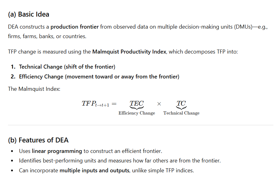
Data Envelopment Analysis (DEA) Method
DEA is a non-parametric, frontier-based approach used to measure TFP and efficiency when multiple inputs and outputs are involved.
It does not require a specific functional form of production and is data-driven.
Basic idea (technical change?)
(c) Advantages of DEA
No need to specify a production function (non-parametric).
Separates technical change from efficiency change—something the index method cannot do.
Works well with cross-sectional data and sectors with multiple outputs (e.g., banks, schools).
Useful when market prices for inputs/outputs are not available.
(d) Limitations of DEA
Sensitive to measurement errors and outliers.
Assumes all deviations from the frontier represent inefficiency.
Does not account for statistical noise.
Requires large datasets for reliability.
Key Differences Between Index Method and DEA
| Basis | Index Method | DEA Method |
|---|---|---|
| Type | Parametric | Non-parametric |
| Purpose | Measures aggregate TFP growth | Measures TFP + efficiency change |
| Data Requirement | Mainly macro time-series | Micro or sectoral cross-sectional data |
| Assumptions | Production function, factor shares | No functional form needed |
| Multiple Outputs | Difficult | Easily handled |
| Noise Handling | Economic theory-based | Sensitive to noise and outliers |
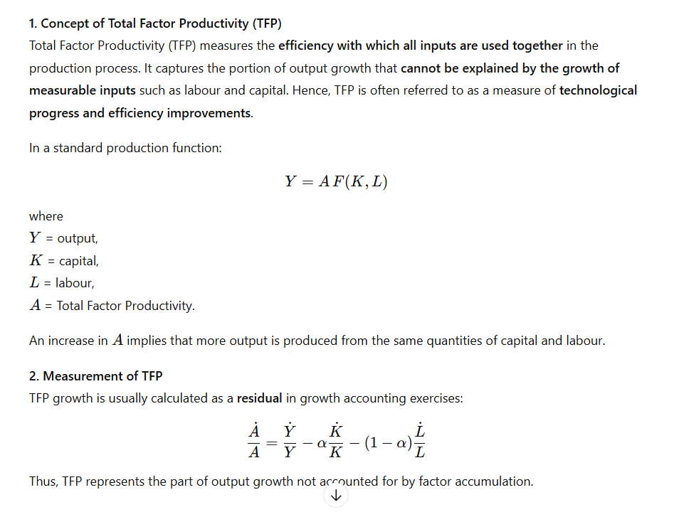
Total Factor Productivity (TFP)
Concept
Factors affecting TFP
1. Technological Progress
Advancements in technology, innovation, research and development (R&D), and adoption of new production techniques significantly enhance productivity.
2. Human Capital and Skills
Education, training, health, and skill development improve workers’ efficiency, adaptability, and ability to use advanced technologies, thereby raising TFP.
3. Institutional Quality and Governance
Efficient institutions, secure property rights, rule of law, low corruption, and effective governance improve resource allocation and productivity.
4. Infrastructure Development
Quality infrastructure such as transport, power, communication, and digital networks reduces transaction costs and improves overall efficiency.
5. Economies of Scale and Learning-by-Doing
Expansion of production leads to cost reductions through experience, specialisation, and learning-by-doing, which positively affects TFP.
6. Trade Openness and Global Integration
Exposure to international markets promotes competition, technology transfer, and better management practices, thereby enhancing productivity.
7. Structural Change
Shifting resources from low-productivity sectors (such as traditional agriculture) to high-productivity sectors (industry and services) raises overall TFP.
8. Financial Development
Efficient financial markets facilitate better allocation of capital to productive uses, encourage innovation, and improve productivity.
9. Macroeconomic Stability
Low inflation, fiscal discipline, and stable economic policies reduce uncertainty and encourage long-term investment, supporting productivity growth.
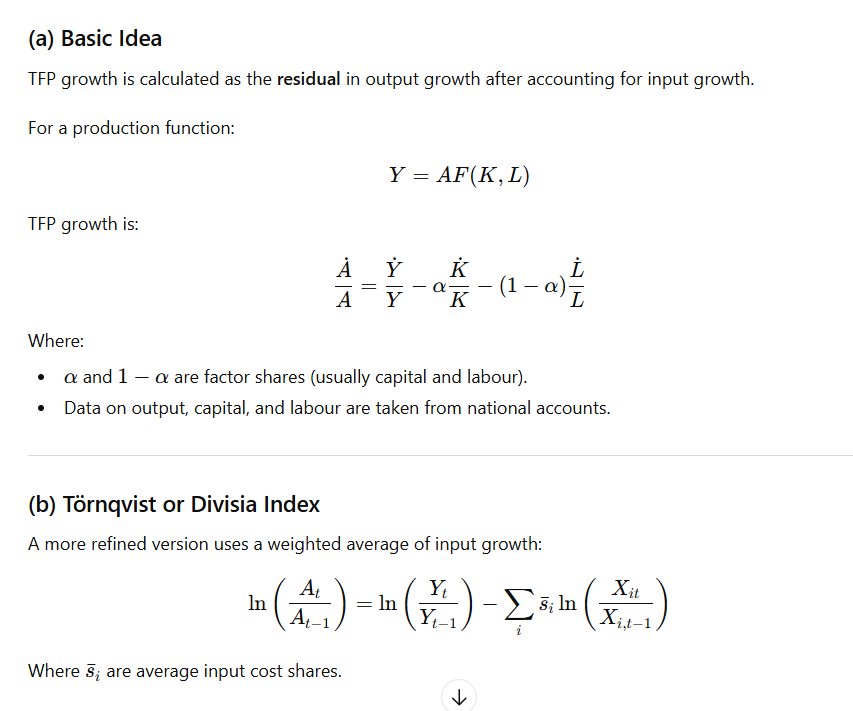
Methods of Measuring Total Factor Productivity
1. Growth Accounting Method (Solow Residual)
Assumes a specific production function (usually Cobb–Douglas)
Measures TFP as the residual after accounting for input growth
Simple and widely used
Limitations:
Sensitive to measurement errors
Assumes perfect competition and constant returns to scale
2. Index Number Approach
Constructs output and input indices
TFP growth = growth of output index − growth of input index
Common indices:
Tornqvist index
Divisia index
Merit: Allows multiple inputs
Limitation: Requires detailed data
3. Data Envelopment Analysis (DEA)
Non-parametric method
Uses linear programming to construct an efficiency frontier
Measures relative efficiency across firms or countries
Merit: No functional form required
Limitation: Sensitive to outliers and noise
4. Stochastic Frontier Analysis (SFA)
Parametric approach
Separates inefficiency from random error
Estimates a production frontier statistically
Merit: Accounts for statistical noise
Limitation: Requires functional form assumption
5. Total Factor Productivity Indices over Time
Malmquist Productivity Index
Decomposes productivity change into:
Efficiency change
Technological change
Widely used in panel data analysis.
How do property rights and transaction costs work to create institutions that influence development?
Institutions—defined as the formal and informal rules that structure economic behaviour—play a central role in shaping development outcomes. Two fundamental concepts in the New Institutional Economics framework, property rights and transaction costs, explain how institutions emerge and why they matter for economic development.
1. Property Rights and Development
Property rights refer to the legally and socially recognised claims individuals or groups have over resources, assets, and returns from their use.
(a) Function of Property Rights
Effective property rights:
Provide security of ownership
Individuals are more willing to invest in land, capital, and businesses when their claims are protected.Create incentives for productive activity
Secure rights ensure people can enjoy the fruits of their labour.Enable exchange and contracting
Clearly defined rights make it easier to trade, mortgage, rent, or use assets as collateral.Support efficient resource allocation
Markets function efficiently only when rights are clear and enforceable.
(b) Impact on Development
Well-defined property rights increase investment, innovation, and entrepreneurship.
They reduce disputes and encourage long-term planning.
Weak property rights result in informality, rent-seeking, and underinvestment.
Land reform or titling programmes often improve credit access and productivity.
Thus, institutional development often begins with securing property rights.
2. Transaction Costs and Development
Transaction costs are the costs of making economic exchanges. They include:
information costs
negotiation and bargaining costs
monitoring and enforcement costs
legal and administrative expenses
High transaction costs make markets inefficient or unworkable.
(a) How Transaction Costs Influence Institutions
Institutions evolve to reduce transaction costs. For example:
Legal systems reduce enforcement costs.
Contracts and norms reduce information asymmetry.
Regulated markets reduce uncertainty in trading.
Financial institutions reduce costs of borrowing and lending.
(b) Impact on Development
Lower transaction costs promote specialisation, trade, and investment.
High transaction costs discourage formal market participation and cause informal arrangements.
Poor governance, corruption, and weak enforcement increase transaction costs, slowing development.
Hence, institutions emerge as mechanisms for making transactions cheaper and more reliable.
3. How Property Rights and Transaction Costs Together Create Institutions
Institutions develop when societies recognise the need to:
Define ownership (property rights)
Reduce the cost of exchange (transaction costs)
Examples:
(a) Courts and Legal Frameworks
Courts enforce contracts and protect rights.
They reduce transaction uncertainty and disputes.
(b) Financial Institutions
- Banks rely on property rights (collateral) and reduce transaction costs in credit markets.
(c) Market Regulations
- Licensing, registration, and standard-setting bodies evolve to reduce transaction-related risks.
(d) Cooperatives and Community Institutions
- Informal institutions arise where formal systems are weak to guarantee rights and lower costs.
(e) Governance and Bureaucratic Institutions
- Land registries, patent offices, and regulatory bodies exist to define, record, and enforce rights efficiently.
Thus, institutions emerge as solutions to economic frictions.
4. Consequences for Economic Development
Higher Efficiency
Secure rights + low transaction costs → efficient markets → higher productivity.More Investment
Investors are more willing to invest when rights are secure and costs of contracting are low.Innovation and Entrepreneurship
Intellectual property rights incentivise innovation.Reduced Corruption and Informality
Strong institutions lower rent-seeking and increase formal participation.Inclusive Growth
Clear rights over land, credit, and resources empower disadvantaged groups.Better Allocation of Resources
Markets allocate land, labour, and capital more efficiently with strong institutions.
Geography impacts development
Geography has long been recognised as a fundamental determinant of economic development. Classical economists, economic historians, and modern development theorists have all emphasised that.
1. Geography as a Starting Condition for Development
Geography provides the initial conditions under which economies begin their development trajectories. These conditions influence:
agricultural productivity
population density
settlement patterns
trade possibilities
institutional evolution
Historical development patterns reveal persistent effects of early geographic advantages or disadvantages.
2. Climate and Agricultural Productivity
Temperate vs. Tropical Regions
Historically, temperate regions experienced:
moderate rainfall
fertile soils
fewer crop diseases
These conditions supported stable agriculture and surplus generation, which enabled urbanisation and specialisation.
In contrast, tropical regions faced:
soil nutrient depletion
pests and plant diseases
rainfall variability
This reduced agricultural surplus and constrained early capital accumulation.
Historical Evidence:
Europe’s agricultural surplus supported medieval towns and later industrialisation.
Many tropical economies remained agrarian with low productivity until modern technology.
3. Disease Environment and Human Capital
Geography strongly influenced disease burden.
Tropical regions had high prevalence of malaria, yellow fever, and sleeping sickness.
These diseases reduced life expectancy, labour productivity, and incentives to invest in education.
Historical Example:
European settlement was limited in high-mortality regions (e.g., Sub-Saharan Africa), affecting colonial strategies and institutional quality.
Acemoglu, Johnson, and Robinson show that disease environments shaped extractive vs. settler institutions.
Thus, disease geography had long-term effects on human capital formation and institutions.
4. Access to Waterways and Trade Routes
Geographic access to navigable rivers, coastlines, and natural harbours historically lowered transportation costs and facilitated trade.
Historical Examples:
River-based civilisations (Indus, Nile, Tigris-Euphrates) flourished due to irrigation and trade.
European coastal nations (Britain, Netherlands) benefited from maritime trade and colonial expansion.
Landlocked regions faced higher transport costs and limited market access.
Trade access allowed:
market expansion
technological diffusion
capital accumulation
These advantages persisted over centuries.
5. Natural Resources and Development
Geography determines resource endowments such as minerals, forests, and energy sources.
Positive Effects:
Coal deposits in Britain enabled the Industrial Revolution.
Oil resources transformed Middle Eastern economies.
Negative Effects (Resource Curse):
- Resource abundance sometimes led to rent-seeking, conflict, and weak institutions.
Thus, geography influences development through both productive and political channels.
6. Geography and Technological Diffusion
Geography affects how easily technologies spread.
Eurasia’s east-west axis allowed similar climates, easing diffusion of crops, animals, and technologies.
Africa and the Americas, with north-south axes, faced ecological barriers to diffusion.
This influenced the pace of agricultural and technological advancement across continents (Jared Diamond).
7. Geography and Institutional Development
Geographic conditions shaped colonial strategies and institutions.
In hospitable regions, Europeans settled and established inclusive institutions.
In disease-prone regions, colonisers set up extractive institutions.
These institutional differences persisted post-independence and continue to influence development.
8. Persistence and Path Dependence
Geographic effects exhibit path dependence:
Early geographic advantages enabled capital accumulation and institutional development.
These, in turn, reinforced growth through feedback mechanisms.
Thus, geography affects development indirectly and historically, rather than deterministically.
9. Limits of Geographic Determinism
Geography is not destiny.
Technological progress (irrigation, vaccines, air conditioning) reduces geographic constraints.
Policy choices, institutions, and human capital can overcome disadvantages.
Examples:
Singapore and Hong Kong prospered despite limited natural resources.
Green Revolution reduced climatic constraints on agriculture in India.
10. Interaction of Geography with Institutions and Policy
Modern development outcomes depend on the interaction of geography with:
institutions
technology
governance
global integration
Geography sets the stage, but institutions determine performance.
Role of the state in economic development
1. Theoretical Perspectives on the Role of the State
(a) Classical and Neoclassical View
The state should play a limited role, confined to:
law and order
property rights protection
national defence
Markets are assumed to be efficient, and state intervention distorts incentives.
(b) Keynesian and Structuralist View
Markets can fail due to unemployment, demand deficiency, and structural rigidities.
The state must actively intervene to:
stabilise the economy
promote investment
guide structural change
(c) Developmentalist State Perspective
Based on East Asian experience (Japan, South Korea, Taiwan).
The state plays a strategic and coordinating role in industrialisation and export promotion.
2. Correcting Market Failures
Markets often fail in developing economies due to:
externalities
public goods
information asymmetry
monopolies
State’s Role
Provision of public goods: infrastructure, roads, ports, power, law and order.
Regulation of monopolies and competition policy.
Intervention in education, health, and R&D due to positive externalities.
Without state intervention, private investment in these areas remains suboptimal.
3. Capital Formation and Infrastructure Development
Developing countries face shortages of capital and long gestation projects.
State’s Role
Mobilisation of savings through taxation and public borrowing.
Direct investment in:
infrastructure
heavy industries
basic manufacturing
Historical Evidence:
Public sector investment was central to industrialisation in India during the Five-Year Plans.
Infrastructure created by the state crowds in private investment.
4. Industrialisation and Structural Transformation
Economic development requires a shift from agriculture to industry and services.
State’s Role
Industrial policy to promote infant industries.
Protection, subsidies, and credit support during early stages.
Coordination of complementary investments (big push argument).
Examples:
East Asian economies used export-oriented industrial policies.
Strategic protection helped build global competitiveness.
5. Human Capital Formation
Markets underinvest in education and health due to long-term returns and externalities.
State’s Role
Public provision of education and healthcare.
Skill development and training programmes.
Nutrition, sanitation, and social infrastructure.
Human capital is essential for productivity growth and technological adoption.
6. Poverty Reduction and Social Welfare
Growth alone does not ensure equitable development.
State’s Role
Social security schemes.
Poverty alleviation programmes.
Employment generation (e.g., public works).
Redistribution through progressive taxation.
The state ensures that development is inclusive and socially sustainable.
7. Macroeconomic Stabilisation
Developing economies are prone to instability.
State’s Role
Fiscal policy to stabilise output and employment.
Counter-cyclical spending during recessions.
Management of inflation and public debt.
Stability is a prerequisite for long-term growth.
8. Institution Building and Governance
Institutions do not emerge automatically.
State’s Role
Establishment of legal systems and contract enforcement.
Protection of property rights.
Reduction of transaction costs.
Regulation of markets and financial systems.
Strong institutions improve investment climate and efficiency.
9. Global Integration and Development
Developing countries face asymmetric global markets.
State’s Role
Managing trade liberalisation.
Negotiating international agreements.
Protecting vulnerable sectors during adjustment.
Promoting exports and technological upgrading.
The state mediates between domestic priorities and global pressures.
10. Limits and Risks of State Intervention
While the state is essential, excessive intervention can cause:
bureaucratic inefficiency
rent-seeking and corruption
misallocation of resources
fiscal stress
This leads to government failure, as seen in inefficient public enterprises and over-regulation.
Hence, the challenge is not “state vs market” but effective state and efficient markets.
11. Changing Role of the State
The role of the state evolves with development stages:
Early stage: active intervention, planning, infrastructure creation.
Middle stage: regulation, coordination, human capital investment.
Advanced stage: facilitation, innovation support, social protection.
Modern development emphasises a capability-enhancing state, not a controlling one.
Impact of Economic Development on the Emergence and Functioning of Democracy
1. Economic Development and the Emergence of Democracy
(a) Modernisation Hypothesis
According to the modernisation theory (Lipset), economic development promotes democracy by:
raising income levels,
increasing literacy and education,
expanding the middle class, and
reducing extreme poverty.
These changes create social conditions favourable to democratic values such as tolerance, participation, and accountability.
(b) Social Structural Changes
Development transforms class structures:
Growth of an urban, educated middle class increases demand for political representation.
Decline of feudal or traditional authority weakens authoritarian control.
Historically, democracies in Western Europe and North America emerged alongside industrialisation.
2. Economic Development and Democratic Functioning
(a) Strengthening Institutions
Economic development provides resources to build:
effective bureaucracies,
independent judiciary,
professional electoral systems.
Stronger institutions enhance democratic governance.
(b) Reduction of Distributional Conflict
Higher incomes reduce zero-sum conflicts over scarce resources, making democratic compromise easier.
(c) Expansion of Civil Society
Development encourages:
media freedom,
voluntary organisations,
interest groups.
These institutions improve citizen participation and oversight.
3. Economic Development and Political Participation
Education increases political awareness and participation.
Economic security enables citizens to engage in politics beyond survival concerns.
Greater communication infrastructure improves information flow and accountability.
Thus, development deepens democratic participation.
4. Limits and Qualifications
Economic development does not guarantee democracy (e.g., authoritarian growth in some countries).
Democracies can emerge in poor societies but may be fragile.
Inequality can undermine democratic functioning even at higher income levels.
Historical, cultural, and institutional factors also matter.
Rural labour market institutions v/s Formal labour markets
1. Nature of Employment
Rural labour markets are dominated by casual, seasonal, and informal employment, mainly in agriculture and allied activities.
Formal labour markets offer regular, contractual employment with defined job roles and continuity.
2. Wage Determination
In rural labour markets, wages are often determined by:
local customs,
social relations (caste, gender),
implicit contracts, and
subsistence considerations.
In formal labour markets, wages are determined by:
productivity,
labour laws,
collective bargaining, and
market demand and supply.
3. Role of Social Institutions
Rural labour markets are embedded in social institutions such as caste, kinship, and patron–client relationships.
Formal labour markets are governed primarily by legal and contractual institutions, largely independent of social identity.
4. Contractual Arrangements
Rural employment often relies on oral, informal, and implicit contracts.
Formal labour markets rely on written contracts, legal enforcement, and standardised terms of employment.
5. Labour Mobility
Rural labour mobility is limited due to:
land ties,
social obligations,
lack of information, and
migration costs.
Formal labour markets allow higher mobility across firms and regions.
6. Job Security and Benefits
Rural workers face high job insecurity, with no social security or employment protection.
Formal workers enjoy benefits such as:
minimum wages,
pensions,
health insurance,
workplace safety regulations.
7. Role of Intermediaries
Rural labour markets often involve intermediaries (landlords, contractors, moneylenders).
Formal labour markets operate through transparent recruitment systems.
8. Information and Transparency
Information about jobs and wages in rural markets spreads through informal networks.
Formal markets rely on advertisements, employment exchanges, and digital platforms.
9. Power Relations
Rural labour markets often display asymmetric power relations, with employers exercising significant control.
Formal labour markets provide mechanisms for grievance redressal and worker representation.
10. State Regulation
State presence and enforcement of labour laws are weak in rural labour markets.
Formal labour markets are more effectively regulated and monitored.
Theory of path dependence
Path dependence is a concept in economics and social sciences which suggests that current outcomes are strongly influenced by historical events, initial conditions, and past choices, even when those choices were made under different circumstances.
1. Meaning of Path Dependence
Path dependence implies that:
History matters in economic outcomes.
Small, random, or temporary events can have long-lasting effects.
The economy does not always converge to a single efficient equilibrium.
Thus, the final outcome depends not only on fundamentals but also on the sequence of events.
2. Origins of the Concept
The idea was popularised by:
Paul David (1985) – study of the QWERTY keyboard.
Brian Arthur (1989) – increasing returns and self-reinforcing processes.
It is widely applied in development economics, institutional economics, and technology adoption.
3. Mechanisms of Path Dependence
(a) Increasing Returns
Early advantages lead to further gains, making one option dominant.
(b) Learning Effects
Users become more skilled with a particular technology over time.
(c) Coordination Effects
The value of a choice increases as more people adopt it.
(d) Adaptive Expectations
People choose options they expect others to choose.
(e) High Switching Costs
Changing to an alternative becomes costly once investments are made.
4. Path Dependence in Economic Development
(a) Institutions
Colonial institutions created long-term effects on governance and growth.
(b) Technology
Early adoption of certain technologies locks economies into specific trajectories.
(c) Industrial Location
Initial location of industries influences future clustering.
(d) Poverty Traps
Historical disadvantages can perpetuate underdevelopment.
5. Implications of Path Dependence
Multiple equilibria are possible.
History and timing matter.
Market outcomes may be inefficient.
Development is uneven across countries.
Policy interventions can alter development paths if timed well.
6. Criticisms
Overemphasis on history may underplay role of rational choice.
Difficult to empirically distinguish from persistence.
Some paths can be reversed with strong institutions and technology.
Increasing Returns, Monopolistic Competition, and Economic Growth
Traditional neoclassical growth models assume constant returns to scale and perfect competition, which imply diminishing returns to capital and limit long-run growth unless technological progress is exogenously given. Modern growth theory departs from this view by emphasising increasing returns to scale and monopolistic competition, which together provide a powerful explanation of endogenous and sustained economic growth.
1. Increasing Returns to Scale
Meaning
Increasing returns to scale occur when a proportional increase in inputs leads to a more than proportional increase in output. This is common in activities involving:
knowledge and ideas
research and development (R&D)
human capital
technology-intensive production
Knowledge is non-rival—its use by one firm does not reduce its availability to others—making increasing returns possible at the aggregate level.
Impact on Economic Growth
Sustained Growth
Increasing returns prevent diminishing returns to capital, allowing growth to continue without slowing down.Knowledge Spillovers
Innovations by one firm raise productivity of others, creating positive externalities that boost overall growth.Cumulative Causation
Early advantages reinforce themselves, leading to persistent growth and divergence across countries.Multiple Equilibria
Economies may settle on different growth paths depending on initial conditions.
Thus, increasing returns are central to endogenous growth.
2. Monopolistic Competition
Meaning
Monopolistic competition is characterised by:
many firms
product differentiation
some degree of monopoly power
free entry in the long run
This market structure is central to modern growth models such as those of Romer and Aghion–Howitt.
3. Role of Monopolistic Competition in Growth
Incentives for Innovation
Firms invest in R&D because temporary monopoly profits reward successful innovation.Product Variety Expansion
Growth occurs through an increase in the number of intermediate goods and product varieties, raising productivity.Endogenous Technological Change
Innovation results from profit-seeking behaviour rather than exogenous forces.Efficient Balance Between Competition and Monopoly
Monopolistic competition allows innovation while maintaining competitive pressure.
4. Interaction Between Increasing Returns and Monopolistic Competition
Increasing returns make perfect competition unsustainable, as firms must cover fixed R&D costs.
Monopolistic competition enables firms to recover these costs through mark-ups.
Together, they:
support continuous innovation,
generate self-sustaining growth, and
explain why growth can be persistent and uneven.
5. Limitations
Monopoly power may lead to inefficiency and inequality.
Excessive protection of intellectual property may reduce competition.
Early models predict scale effects that are not always observed empirically.
Economic Growth vs Economic Development
Meaning
Economic growth refers to a quantitative increase in a country’s output or income over time. It is usually measured in terms of increase in real national income, real GDP, or per capita income.
Economic development, on the other hand, is a broader and qualitative concept. It includes not only growth in income but also structural, institutional, social, and technological changes that improve the overall quality of life of the people.
Thus, economic growth is a necessary but not sufficient condition for economic development.
Distinction between Economic Growth and Economic Development
| Basis | Economic Growth | Economic Development |
|---|---|---|
| Nature | Quantitative | Qualitative and quantitative |
| Scope | Narrow concept | Broad and comprehensive concept |
| Focus | Increase in output/income | Improvement in living standards |
| Measurement | GDP, GNP, per capita income | HDI, poverty, literacy, health, inequality |
| Structural change | Not necessary | Essential |
| Income distribution | Ignored | Considered important |
| Time horizon | Short to medium term | Long-term process |
| Welfare aspect | Not explicitly included | Central objective |
Economic growth may occur without development, for example when income rises but poverty, inequality, unemployment, and poor health conditions persist, as seen in many developing countries.
Indicators of Economic Development
Economic development is multidimensional and cannot be measured by a single indicator. The important indicators are discussed below:
1. Per Capita Income
An increase in real per capita income indicates improved average material well-being. However, it is an incomplete indicator as it does not reflect income distribution or non-economic aspects of welfare.
2. Structural Change
Development involves a shift in:
Output and employment from agriculture to industry and services
Traditional techniques to modern technology
Informal sector to formal sector
Structural transformation is a key feature of sustained economic development.
3. Poverty Reduction
Decline in:
Headcount poverty ratio
Poverty gap
Multidimensional poverty
A reduction in absolute and relative poverty indicates that growth is inclusive.
4. Income Distribution and Inequality
Improvement in income distribution measured through:
Gini coefficient
Lorenz curve
Development requires that the benefits of growth are equitably shared.
5. Human Development Indicators
Introduced by UNDP, Human Development Index (HDI) includes:
Life expectancy (health)
Education (mean and expected years of schooling)
Per capita income (PPP)
HDI captures development beyond income.
6. Health Indicators
Life expectancy at birth
Infant Mortality Rate (IMR)
Maternal Mortality Rate (MMR)
Better health outcomes indicate improved quality of life and productivity.
7. Educational Indicators
Literacy rate
School enrolment ratios
Years of schooling
Education enhances human capital and long-term growth potential.
8. Employment and Quality of Employment
Reduction in unemployment and underemployment
Shift from casual to regular and productive employment
Development requires productive employment, not just job creation.
9. Social and Institutional Indicators
Access to basic services (water, sanitation, housing)
Gender equality
Social mobility
Quality of governance and institutions
Strong institutions support sustainable development.
10. Environmental Sustainability
Sustainable use of natural resources
Control of pollution and ecological degradation
Development must be environmentally sustainable, not growth at the cost of future generations.
Vicious Circle of Poverty
The vicious circle of poverty refers to a situation in which poverty perpetuates itself through mutually reinforcing economic and social factors, making it difficult for an economy or individuals to escape from low levels of income and development.
The concept was prominently discussed by Ragnar Nurkse, who argued that poverty is both a cause and a consequence of underdevelopment.
1. On the Supply Side (Low Productivity)
Low income →
Low savings →
Low investment →
Low capital formation →
Low productivity →
Low income
This cycle continues, trapping the economy at a low level of output.
2. On the Demand Side (Low Market Size)
Low income →
Low purchasing power →
Small market size →
Low inducement to invest →
Low productivity and output →
Low income
Thus, both supply and demand constraints reinforce poverty.
3. Human Capital Aspect
Low income →
Poor nutrition, health, and education →
Low labour efficiency →
Low productivity →
Low income
This creates intergenerational transmission of poverty.
Measures to break from it
1. Capital Formation and Investment
Increase domestic savings
Promote public investment in infrastructure
Encourage private and foreign investment
This raises productive capacity.
2. Big Push and Balanced Growth
Simultaneous investment in multiple sectors
Expansion of market size
Overcomes demand-side constraints
3. Human Capital Development
Investment in education, health, and skill development
Improved nutrition and sanitation
Enhances productivity and earning capacity.
4. Technological Progress
Adoption of modern technology
Productivity improvement in agriculture and industry
Raises output without proportionate increase in inputs.
5. Employment Generation
Labour-intensive industrialisation
Rural development and non-farm activities
Provides income and demand stimulus.
6. Institutional Reforms
Land reforms
Access to credit
Financial inclusion
Reduces structural inequality and exclusion.
7. Government Intervention
Public works programmes
Social security schemes
Targeted poverty alleviation programmes
Helps the poor escape subsistence-level income.
Demographic transition in developing economies
Demographic transition refers to the historical process through which a country moves from a regime of high birth rate and high death rate to one of low birth rate and low death rate, accompanied by changes in population growth and age structure.
Stage I: High Birth Rate and High Death Rate
Characteristic of traditional societies
Poor health facilities and low life expectancy
Population growth is slow
(Most developing countries have already passed this stage.)
Stage II: High Birth Rate and Declining Death Rate
Improvement in medical facilities and sanitation
Death rate declines rapidly
Birth rate remains high due to social and cultural factors
Leads to population explosion
Most developing economies experienced this stage during the early phases of development.
Stage III: Declining Birth Rate and Low Death Rate
Increased urbanization and education
Rising female literacy and employment
Use of contraception
Population growth rate begins to slow
Many developing countries, including India, are currently in this stage.
Stage IV: Low Birth Rate and Low Death Rate
Stable population
High level of development
Found mainly in developed economies
Characteristics of Demographic Transition in Developing Economies
Rapid population growth during Stage II
Declining mortality without a corresponding decline in fertility
High dependency ratio
Pressure on resources, employment, and social services
Potential for demographic dividend if properly managed
Importance of Population Policy in This Context
1. Controlling Population Growth
Population policy helps reduce fertility rates through:
Family planning programmes
Awareness campaigns
This prevents strain on economic resources.
2. Improving Human Capital
Policies promoting:
Education (especially female education)
Health and nutrition
Accelerate the fertility transition and raise productivity.
3. Realising Demographic Dividend
By:
Skill development
Employment generation
Population policy converts a large working-age population into an economic asset.
4. Reducing Dependency Burden
Lower fertility reduces the proportion of dependents, improving savings and investment capacity.
5. Promoting Gender Equality
Population policies encouraging:
Women’s empowerment
Delayed marriage
Have long-term demographic and economic benefits.
6. Sustainable Development
Population stabilization supports:
Environmental sustainability
Better access to housing, water, and health services
Export-led growth
Export-led growth (ELG) is a development strategy in which economic growth is driven by expansion of exports. The strategy emphasizes:
Production for foreign markets
Specialization based on comparative advantage
Integration with the global economy
According to this approach, exports act as an engine of growth by stimulating output, employment, productivity, and technological progress.
Mechanism of Export-Led Growth
Export-led growth promotes development through the following channels:
Increase in Aggregate Demand
Exports raise effective demand, leading to higher output and income.Foreign Exchange Earnings
Export earnings finance imports of capital goods, technology, and raw materials.Economies of Scale
Access to international markets allows firms to expand production and reduce costs.Technological Upgradation
Exposure to global competition encourages efficiency and innovation.Employment Generation
Export-oriented industries absorb labour, especially in manufacturing and services.
India’s Growth Strategy in the Context of External Trade
1. Pre-1991: Import Substitution Strategy
Before 1991, India followed an import-substitution industrialisation (ISI) strategy characterized by:
High tariffs and quantitative restrictions
Export pessimism
Focus on domestic markets
Exports grew slowly, foreign exchange shortages were frequent, and integration with the world economy remained limited.
2. Post-1991: Shift towards Export Orientation
After the New Economic Policy (1991), India gradually adopted elements of an export-led growth strategy:
Trade liberalisation
Reduction in tariffs
Removal of quantitative restrictions
Market-determined exchange rate
Promotion of export-oriented units (EOUs) and SEZs
India’s Current Strategy: Balanced Approach
Recent initiatives reflect a calibrated approach:
Make in India
Production-Linked Incentive (PLI) schemes
Export promotion coupled with domestic capacity building
India is moving towards a mixed strategy combining:
Export promotion
Domestic demand-led growth
Strategic protection where necessary
Consequences of climate change for the economy
Climate change refers to long-term changes in temperature, rainfall patterns, and the frequency of extreme weather events caused largely by human activities. Its economic consequences are wide-ranging and affect both developed and developing economies, particularly in the long run.
1. Impact on Agriculture and Food Security
Climate change adversely affects agricultural productivity through irregular rainfall, rising temperatures, droughts, floods, and soil degradation. Crop yields decline, production becomes more uncertain, and food prices rise, leading to food insecurity, especially in agrarian and developing economies.
2. Effects on Economic Growth
Frequent climate shocks reduce overall economic growth by destroying productive assets, disrupting production, and lowering labour productivity. Developing countries face greater growth losses due to their dependence on climate-sensitive sectors such as agriculture and fisheries.
3. Employment and Livelihoods
Climate change threatens employment in agriculture, forestry, fisheries, and tourism. Loss of livelihoods leads to increased poverty, informal employment, and rural–urban migration, placing pressure on urban infrastructure and labour markets.
4. Impact on Health and Human Capital
Rising temperatures and extreme weather increase the incidence of diseases, heat stress, and malnutrition. Poor health reduces labour productivity, increases healthcare expenditure, and weakens human capital formation, affecting long-term economic development.
5. Infrastructure Damage and Public Finance
Extreme weather events such as floods, cyclones, and heatwaves damage infrastructure including roads, power systems, housing, and communication networks. Governments face higher fiscal burdens due to increased spending on disaster relief, rehabilitation, and adaptation measures.
6. Inequality and Poverty
Climate change disproportionately affects the poor, as they have limited capacity to adapt and rely heavily on natural resources. Income inequality widens, and poverty levels increase due to loss of assets, employment, and access to basic services.
7. External Sector and Trade
Climate-induced disruptions affect exports of agricultural and natural-resource-based goods. Rising import dependence for food and energy worsens balance of payments and exposes economies to international price volatility.
8. Financial Stability and Investment
Climate risks increase uncertainty, discourage private investment, and raise insurance costs. Financial institutions face higher credit risks, while governments need to mobilise large resources for climate mitigation and adaptation.
9. Long-term Development Challenges
Climate change constrains sustainable development by diverting resources from growth-enhancing investments to coping and adaptation measures. It also threatens progress towards development goals such as poverty reduction and food security.
Learning-by-doing model of Kenneth Arrow.
Kenneth Arrow’s learning-by-doing model (1962) is an important contribution to growth theory. It explains technological progress as an outcome of experience gained in the process of production, rather than as an exogenously given factor.
1. Basic Idea
Arrow argued that productive efficiency improves as cumulative production increases. Workers, firms, and managers learn from past production activities, leading to better methods, reduced costs, and higher productivity. Thus, learning is a by-product of investment and production.
2. Endogenous Technological Progress
Unlike the Solow model where technical progress is exogenous, Arrow’s model treats technological change as endogenous. Knowledge accumulation results automatically from investment in capital and expansion of output.
3. Role of Capital Accumulation
In the model, new capital embodies improved technology. As firms invest more and capital stock rises, experience accumulates, leading to higher labour productivity. Hence, capital accumulation generates increasing efficiency over time.
4. Externalities of Learning
Learning-by-doing generates positive externalities. Knowledge created by one firm spills over to others and becomes a public good. Since firms cannot fully appropriate the benefits of learning, private investment may be lower than socially optimal.
5. Production Function Representation
Arrow expressed learning through a production function where productivity depends on cumulative investment or output:
$$Y = A(K) , F(K, L)$$
Here, A(K)A(K)A(K) increases with cumulative capital stock, capturing the learning effect. As KKK grows, productivity rises even if conventional inputs remain unchanged.
6. Implications for Returns to Scale
Although individual firms may face constant returns to scale, the economy as a whole may experience increasing returns to scale due to learning externalities. This helps explain sustained economic growth without diminishing returns.
7. Path Dependence and Growth
The model highlights path dependence: economies that invest and industrialise early gain more learning benefits and grow faster, while late starters may lag behind without policy support.
8. Policy Implications
Since learning-by-doing is associated with externalities, Arrow’s model provides justification for government intervention, such as subsidies to investment, protection of infant industries, and support for industrialisation and skill formation.
9. Relevance to Developing Economies
The model is particularly relevant for developing countries, where expanding manufacturing and investment can generate rapid productivity gains through experience and learning.
Chinese economy in the pre-reform period (1953-1978)
Performance of the Chinese Economy in the Pre-Reform Period (1953–1978)
The pre-reform period of the Chinese economy covers the years from the First Five-Year Plan in 1953 up to the launch of economic reforms in 1978. This phase was characterized by a centrally planned socialist system inspired largely by the Soviet model.
1. Strategy of Development
China adopted a strategy of central planning with emphasis on heavy industry. The state owned and controlled major means of production, and economic decisions regarding output, prices, investment, and resource allocation were made through Five-Year Plans. Agriculture was collectivized, and private enterprise was virtually eliminated.
2. Growth Performance
During 1953–78, China achieved moderate to fairly high growth of national income, averaging around 5–6 per cent per annum. Industrial output, particularly in heavy industries such as steel, coal, machinery, and chemicals, grew rapidly. However, growth was uneven and unstable, marked by sharp fluctuations due to policy mistakes and political movements.
3. Industrial Development
The pre-reform period witnessed significant industrialisation. China created a broad industrial base from a predominantly agrarian economy. Large-scale investments in infrastructure, basic industries, and state-owned enterprises laid the foundation for future industrial growth. However, industrial production was often inefficient, with low productivity and poor quality due to lack of competition and distorted price incentives.
4. Agricultural Performance
Agriculture performed relatively poorly compared to industry. Collectivisation under People’s Communes reduced incentives for farmers. The Great Leap Forward (1958–61) led to disastrous outcomes, including a massive famine and sharp fall in agricultural output. Although agriculture recovered somewhat in the 1960s and 1970s, productivity remained low and food shortages persisted.
5. Employment and Social Indicators
Despite economic inefficiencies, China made notable progress in human development. There were improvements in literacy, basic education, public health, and life expectancy. Employment was largely guaranteed under the socialist system, though this resulted in disguised unemployment and low labour productivity.
6. External Sector
China followed a policy of self-reliance with limited integration into the world economy. Foreign trade was minimal, technology imports were restricted, and the economy remained largely closed. While this reduced dependence on foreign capital, it also limited access to modern technology and global markets.
7. Political Disruptions
Economic performance was adversely affected by major political campaigns such as the Great Leap Forward and the Cultural Revolution (1966–76). These movements disrupted production, education, and administration, leading to inefficiency and stagnation in several years.
8. Overall Assessment
In summary, the pre-reform period enabled China to achieve basic industrialisation, national unity, and improvements in social indicators, but at the cost of economic inefficiency, low agricultural productivity, and technological backwardness. These limitations ultimately highlighted the need for economic reforms, which were initiated in 1978.
Human Development Index (HDI)
The Human Development Index (HDI) was introduced by the United Nations Development Programme (UNDP) in 1990 to provide a broader measure of development beyond income.
HDI combines three dimensions:
Health – measured by life expectancy at birth
Education – measured by mean years of schooling and expected years of schooling
Standard of living – measured by Gross National Income (GNI) per capita (PPP)
Each dimension is normalized, and the HDI is calculated as the geometric mean of the three indices. HDI highlights the importance of human well-being, capabilities, and quality of life, rather than economic growth alone.